Abstract
This paper presents a fine-grained and multi-sourced dataset for environmental determinants of health collected from England cities. We provide health outcomes of citizens covering physical health (COVID-19 cases, asthma medication expenditure, etc.), mental health (psychological medication expenditure), and life expectancy estimations. We present the corresponding environmental determinants from four perspectives, including basic statistics (population, area, etc.), behavioural environment (availability of tobacco, health-care services, etc.), built environment (road density, street view features, etc.), and natural environment (air quality, temperature, etc.). To reveal regional differences, we extract and integrate massive environment and health indicators from heterogeneous sources into two unified spatial scales, i.e., at the middle layer super output area (MSOA) and the city level, via big data processing and deep learning. Our data holds great promise for diverse audiences, such as public health researchers and urban designers, to further unveil the environmental determinants of health and design methodology for a healthy, sustainable city.
Background & Summary
As urbanization progresses, millions of people have flocked to cities. It is reported that nowadays more than 55% of the world’s population lives in urban areas. A good environment is crucial to healthy and sustainable cities1,2,3,4, yet, air pollution5, deteriorating climates6,7,8, unavailability of public green spaces9,10,11,12, inadequate water, sanitation and hygiene13 are continuously threatening the citizens’ health. As an example, the poor air quality in the UK caused nearly 29,000 deaths and an associated loss of population life of 340,000 life year lost in 200814. Besides, unhealthy lifestyle caused by easy access to alcohol and the lack of green or blue spaces in cities also yields notably negative effects on citizens’ physical and mental health15,16. Collectively, non-communicable diseases account for nearly 70% of global deaths each year before the COVID-19 outbreak1,17. To achieve the United Nations’ Sustainable Development Goals to “make cities and human settlements inclusive, safe, resilient and sustainable”, and “ensure healthy lives and promote well-being for all at all ages” by 203018, in-depth understanding of the correlation between city environment and public health towards better urban planning and retrofit is of critical importance.
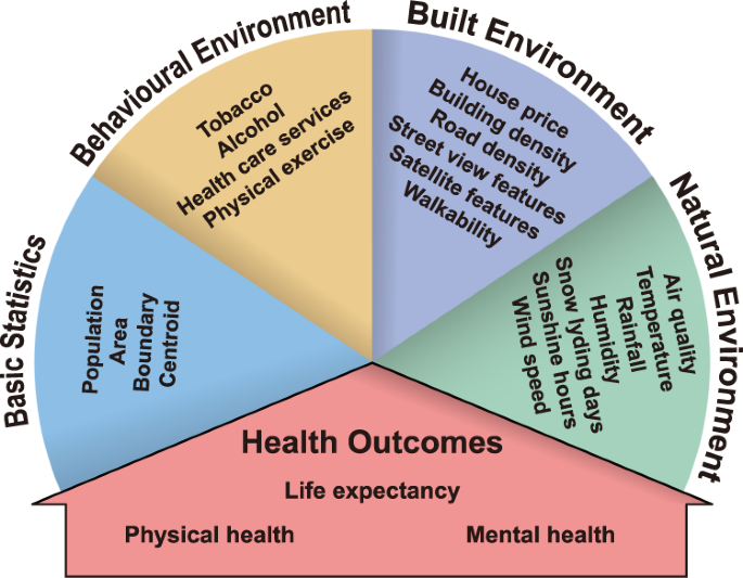
However, a fine-grained and multi-sourced dataset covering heterogeneous environmental determinants of health that can support such studies is lacking. Previous publicly available data usually focus on specific environmental features, such as air pollution19,20,21, tobacco and alcohol accessibility22, or spatial distribution of health services23, which are scattered in different countries with varying spatial resolution. For copyright-protected databases such as UK Biobank24, much effort is still needed to merge the heterogeneous data. The scattered, messy-formatted data significantly increase the cost of research communities, where researchers have to do repetitive works to leverage these data. The high cost of scientific research has incurred public criticism, increasing the tension situation between research communities and taxpayers25. To bridge the data gap between the urban environment and the health outcome of citizens and the social gap between data sources and researchers, we present a comprehensive fine-grained health dataset of 1039 MSOAs in 29 England cities from 2019 to 2022. The topology of the dataset is illustrated in Fig. 1. It consists of two major components: the health outcomes of citizens and the corresponding environmental determinants. For the health outcomes of citizens, we consider the macroscopic life expectancy and the microscopic expenditures of several non-communicable physical and mental diseases. Since the outbreak of COVID-19 at the end of 2019, it has become the most representative communicable disease sweeping the whole world. Thus, we collect fine-grained COVID-19 cases to demonstrate the resilience of cities for pandemics26,27. For the environmental determinants, we adopt a hierarchical view from behavioural factors to natural environments2,4, where the recent advances in deep learning technology and big data processing provide the valuable opportunity to extract environmental determinants of health from heterogeneous data sources such as the road network, street view images and prescription records. Different from previous studies, we provide a unified comprehensive dataset to unmask the border picture of healthy cities.
Overall, this study aims to minimize the social costs to collect and generate fine-grained environmental determinants of health in urban spaces for both public health researchers and urban designers, who might not have the experience to process such heterogeneous big data. Providing a unified dataset and disclosing the data collection and generation processes promote the knowledge discovery in a cost-efficient manner, where the underlying higher-order linkages between multiple environmental factors with diseases can be further investigated through the provided data, and the derived urban patterns can also serve as indicators that shed light on the design of healthy, sustainable cities.
Methods
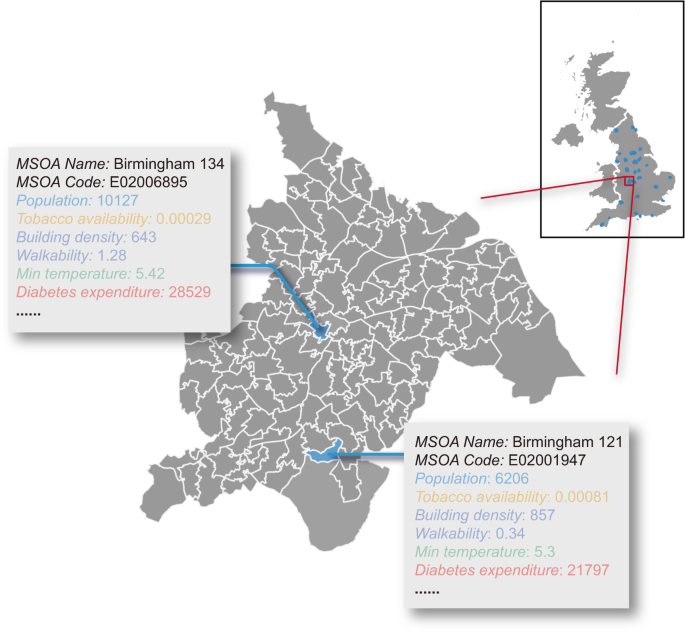
Environmental determinants of health refer to regional, national, and local environmental factors that influence human physical, chemical, and biological health, and all related behaviours. To ensure the comprehensive coverage of various environmental factors, we select basic, behavioural, built, and natural environment descriptors (see Fig. 1 for details). The generation of the target dataset requires heterogeneous data collection, processing, and aggregation, which transforms the input data sources in Table 1 to the unified format illustrated in Fig. 2. We first introduce the determination of geographical units for the target dataset, then discuss the detailed generation process of each subsection of the dataset in Fig. 1.
Determining the geographical units
We select the city-of-interests according to the honour list of city status by the UK government28 and the Office for National Statistics (ONS) Geography definition of major towns and cities29, which captures the high status from both the cultural and economic perspectives. We further filter the cities with administrative power as lower tier local authorities (LTLAs), combining which we acquire 29 representative cities in England (see Table 2 for details).
Datasets from heterogeneous sources often have different geographies: administrative geography, census geographies, postal geography, etc. A unified, fine-grained unit is of great importance to merge these data and unmask the relationship between environmental factors and their health outcomes, so as to support region-level comparisons30. Therefore, we select middle layer super output areas (MSOAs) as the main geographical unit in our study, which is a fine-grained census division that has a mean population of around 7200. As an illustrative example, we visualize the MSOAs of Birmingham city with valid data records in Fig. 2. As a more aggregated point-of-view, we also provide city-level aggregations in our dataset.
To merge collected data in different geographies, we collect MSOA-city lookup table31 and postcode-MSOA lookup table32 from the ONS Geography. By filtering and merging the collected lookup tables according to the city list, we generate a unified geography lookup table as shown in Table 3, which contains 1039 MSOAs. Those identified MSOAs are referred to as the minimum spatial units for our following data processing from all sources, which is used in the following generation procedures to merge the data.
Processing of health outcomes data
We formulate the health outcome of citizens for each region from three aspects: life expectancy, physical health, and mental health. For life expectancy data, we collect gender-specific life expectancy and healthy life expectancy in MSOA level from ONS33, then filter the regions according to the geography lookup table described in Table 3. For physical health, we consider 6 common non-communicable diseases in cities: asthma, cancer, dementia, diabetes, hyperlipidemia, hypertension and obesity. For mental health, we mainly consider depression, psychosis and related disorders in cities. To accurately assess the severity of these diseases, we collect fine-grained prescribing data from the National Health Service (NHS) Business Services Authority34, which serves as an informative data source to estimate the health status of citizens. It contains the drug code, drug quantity, and corresponding expenditure for each practice such as a general practitioner (GP), out-of-Hours service, or a hospital department. Specifically, we focus on expenditure records since they can be used to comprehensively evaluate the severity of diseases across different drugs. Considering the large quantity of the data, we use the Open Data Portal Application Programming Interface (API)35 to query the required information. We filter their corresponding drug codes for physical health and mental health through the British National Formulary (BNF)36. Then we generate the corresponding structured query language (SQL) request through the API to acquire the aggregated actual cost data of these diseases in the postcode level. Since the outbreak of SARS-CoV-2 virus at the end of 2019, COVID-19 has become the most influential communicable disease in urban spaces. We also consider COVID-19 as a representative communicable disease affecting the physical health. For the COVID-19 data, we collect the MSOA level time series from the UK government37, which contains the number of new cases within rolling 7-day periods. During the post process, we merge them into MSOA and city level according to the geography lookup table.
Processing of basic statistics data
The basic statistics data include the population, area, boundary and centroid of selected regions, providing essential information to understand the composition of urban spaces. Specifically, we collect the latest estimates of the usual resident population for MSOA level38, which is in mid-2020. We filter the population numbers of selected MSOAs38 and aggregate them to obtain the city population according to the geography lookup table. The up-to-date city boundary is defined in 201529, which corresponds to the census result of 2011. Thus, we collect the geographical boundary39,40 and the geographical lookup table31,32 of MSOA in their 2011 definition. We adopt the generalized boundary within 20 m error range in our dataset, which strikes a good balance between accuracy and data size. For the boundary data, we filter the MSOA boundary39 and city boundary29 accordingly, and save the polygons in GeoJSON format with the corresponding MSOA codes and city codes. We preserve the original coordinate system of WGS84 in the resulting files. The above boundary data contain the area information of each region, where we modify the data unit into km2 level. According to the population data and area data, we calculate the population density of each MSOA and city in our dataset. For the centroid data, we use the Python packet shapely to calculate the geometric centroids according to the above boundary of cities and MSOAs.
Processing of behaviour environment data
The venues in cities affect the behaviour of citizens in a subtle way, where researchers have demonstrated strong evidence that the availability of tobacco & alcohol22, open green spaces9,10,41, and medical resources42 affect the health outcomes. Here, we focus on the availability of tobacco, alcohol, physical exercise, health care services in a neighbourhood through point-of-interest (POI) data as important health-related behaviour factors. Specifically, we collect the SafeGraph Places Data Schema43, which contains more than 1.5 million records for the whole UK. We filter the POIs by their categories, which are in North American Industry Classification System (NAICS)44 2017 version. NAICS is a classification system developed by the US Census Bureau, which uses a numeric code up to 6 digits in length to hierarchically classify different venues. For tobacco availability, we filter the POIs with NAICS categories of Tobacco Stores and Grocery Stores. We also calculate alcohol availability by Drinking Places, Beer, Wine, Liquor Stores, and Grocery Stores. For physical exercise availability, we consider Fitness and Recreational Sports Centers, Nature Parks and Other Similar Institutions. For health care services availability, we consider Health and Personal Care Stores, Ambulatory Health Care Services, Hospital, Nursing and Residential Care Facilities. Finally, we calculate the availability indicators by the fraction of corresponding POI numbers and region population.
Processing of built environment data
Urban built environment, as an important determinant of health, shapes citizens’ physical activity and mental well-being45. In this study, we incorporate house price, building density, road network density, street view features, satellite features, and walkability to jointly describe the built environment of urban spaces.
We collect the median and mean house price data from ONS46,47,48,49, which include seasonally time series of MSOA level house prices from 1995 until now for both newly built and existing dwellings. It contains common house types such as detached houses, semi-detached houses, terraced houses, flats and manisonettes. Here, we extract the general indicator containing all sales and all house types for the selected regions in our study.
We collect the building information and road networks from OpenStreetMap50. To export large-scale map data, we use the bulk download service provided by Geofabrik51. We manually download the minimal subregion files that contain the city-of-interests, and use the Python packet pyrosm to extract the building information and road networks in interested cities and MSOAs by specifying corresponding boundary polygons. We count the number of buildings in each region, and calculate the building density by dividing it by the area size. For the road network, we filter the driving network, cycling network and walking network accordingly, and calculate the road density indicator by the ratio of total road length and the area size.
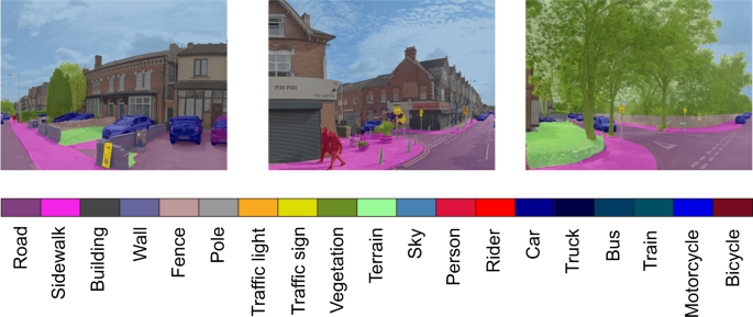
The availability of street view imagery provided by map platforms such as Google52 enables a new angle to observe and analyse the urban environment for the health outcomes for every citizen53,54. For the street view image data, we sample the urban spaces into 100 m × 100 m grids and download the 360° images from Google Map52, which generates 784 thousand images. With the recent advantages of deep learning technology, automatic feature extraction for large-scale image data is possible. In our study, we adopt the state-of-the-art semantic segmentation model ViT-Adapter55 based on vision transformer technology to automatically infer the objects in the street view images, which provides high-accuracy pixel-level classification to the input images. Specifically, we use the official implementation56 provided by the authors trained on Cityscapes dataset57 for our street view images. It recognizes 19 different objects in the image, which are shown in Table 4. We calculate the pixel-level percentage of each objects, and aggregate them in the MSOA and city level to capture the visual semantics of neighbourhood features.
The satellite view imagery is obtained from Esri World Imagery58 according to the method described in59 and its corresponding code implementation60. Specifically, we collect 0.6 m resolution satellite image data tiles covering all the city-of-interests. Then we train the ViT-Adapter55 model on LoveDA dataset61 to extract the 7 labeled objects as features from the collected satellite images. Like the street view images, we aggregate the inference result images according to the MSOA and city boundaries, and calculate the pixel-level percentage of each annotated object.
Walkability is a long-standing indicator in the field of urban planning, which evaluates the mixed-use of amenities to quantify how walking-friendly a neighbourhood is62. In this study, we focus on the health benefit of walkability according to30, which defines walkability as the average z-score of population density, intersection density and a daily living score. We calculate the intersection density through the above OpenStreetMap walking road network data, where we use Python packet shapely to determine whether two roads have any intersection. We summarize the number of intersections in each region, and divide by the corresponding area size as the intersection density. For the daily living score, we consider the density of daily living POIs in each region. According to30, we define daily living POIs in the following categories: Grocery Stores, Nature Parks and Other Similar Institutions, Air Transportation, Rail Transportation, Water Transportation, Transit and Ground Passenger Transportation, and calculate the daily living score by dividing the total number of these POIs with the area size. We normalize the above three indicators according to the following equation
where x* could be the population density, intersection density or daily living score, and μ, σ are the mean and standard variation of x*. Finally, we derive the walkability score by taking the average of normalized indicators.
Processing of natural environment data
Exposure to polluted air is considered a major health challenge for citizens63,64,65. The air quality data is obtained from UK Air66, which is organized by the Department for Environment Food & Rural Affairs (DEFRA). We focus on the Automatic Urban and Rural (AURN) monitoring network, which is the UK’s largest automatic monitoring network for common air pollutants. Specifically, we collect the daily mean records of nitrogen oxides as nitrogen dioxide, PM2.5, and PM10 particulate matter as the air pollution indicators in our dataset. The collected data are available at the station level. We manually select the stations and the corresponding pollution data according to the interactive map67 and station information68. Specifically, for cities with multiple stations, we preserve all the observations in our data.
Climate issue ties tightly with the well-being of all the people69,70,71. Recently, new evidence shows that worsening climate is correlated with a variety of health outcomes, including insufficient nutrition, pandemic outbreaks, and increasing of anxiety and depression72,73. To evaluate how the changing weather affects the health outcome in each region, we collect the weather data from HadUK-Grid maintained by Met Office74, which is a collection of gridded climate variables in high spatial resolution. We collect temperature, precipitation, relative humidity, sunshine duration, snow lying days, and wind speed as the weather features. During the post process, we align the grid data of weather into MSOA and city level. Specifically, we use Python packet h5netcdf to read the weather data, which are provided in NetCDF format. Then we calculate the distance between the gridded data point with the geometric centre of each region by Python packet haversine, and match the nearest one as the target. Considering the size of MSOA and cities, we use 1 km × 1 km resolution data to match each MSOA, and 12 km × 12 km data to match each city.
Data Records
The produced dataset is publicly available through the Figshare repository75, and a live version with potential updates is available in the GitHub repository (https://github.com/0oshowero0/HealthyCitiesDataset). To facilitate data access and utilization, we organise the dataset into several subsections (see Fig. 1). Specifically, the samples of life expectancy data, physical & mental health data, basic statistics data, behavioural environment data, built environment data, natural environment data and health outcomes data are demonstrated in Tables 5–10 accordingly. It provides convenience to researchers who only hope to access part of the data by reducing the data loading time.
All the data are available in tabular format, where the MSOA codes or city codes are used to correlate different subsections of the data. We provide the geographic lookup table demonstrated in Table 3 for users who are interested in larger geographical scales such as LTLA or UTLA level. For the life expectancy data in Table 5, we provide gender-specific life expectancy and healthy life expectancy with 95% confidence intervals. For the physical health and mental health data in Table 6, we provide monthly expenditures per citizen for asthma, cancer, dementia, diabetes, hyperlipidemia, hypertension, obesity, and general mental disorders. For the COVID-19 data, we provide new cases time series in a 7-day rolling window, which is available on a weekly basis. For the basic statistics in Table 7, we have population, area size, population density, geographical centroid, and boundary polygon information. The area size is available in km2, and the centroid data and boundary are available in WGS84. The behaviour environment in Table 8 contains the availability of tobacco, alcohol, health service, and physical exercise POIs by the corresponding POI number divided by the population size. For the built environment in Table 9, we provide building density, median/mean house price, driving/cycling/walking road density, street view features, satellite features, and walkability score. The building density represents the number of buildings per km2, and the house price data are available on a quarterly basis. The road density data represents the average road length (in km) per km2. The street view and satellite view features demonstrate the average percentage of each visual element in the image data. Walkability represents the average z-score of population density, intersection density and daily living score. For the natural environment in Table 10, we provide the NOx, PM2.5, PM10 indices (ug/m3), min/max temperature (°C), rainfall (mm), relative humidity (%), snow lying days (days per month), sunshine hours (hours per month), and wind speed (knots). Except for the snow lying days, sunshine hours and wind speed that are available in a monthly basis, all other natural environment data are available on a daily basis.
Intensive correlations between environmental factors and health outcomes can be discovered through the data records. For instance, the availability of bars is linked with alcohol-related harms22,23, which can be evaluated through the alcohol availability in Table 8 with the drug expenditure in Table 6. Recent studies also demonstrate that street view images are predictive for COVID-19 infections, obesity, diabetes, mental distress, etc.53,54, which can be evaluated through the street view features in Table 9. Besides, researchers can also validate the building and road densities in Table 9 with dementia expenditure to validate their influence on cognitive function41,76. For the natural environment data in Table 10, we can correlate the air pollution data with the expenditure for mental disorders in Table 6 to validate the effect on psychopathology65, or investigate the influence of temperature and other weather features for citizens’ health72,73. Furthermore, our data provide an opportunity to investigate the high-order correlation between various environmental factors and health outcomes, which is still an unresolved research question. Consequently, our produced data will benefit and facilitate a plethora of related studies.
Technical Validation
Representativeness of selected cities
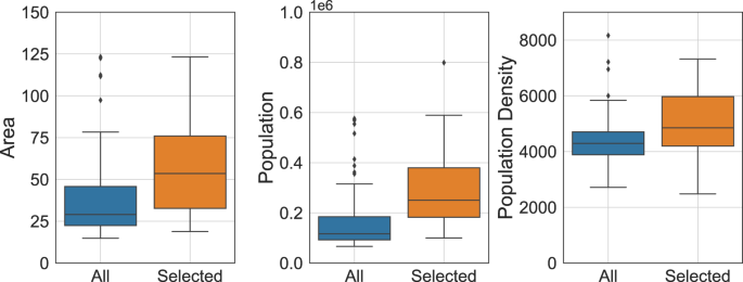
In this study, we select representative England cities according to the availability of the source data, where cities that have high status in economic, political and cultural perspectives have been included in our dataset. In Fig. 3, we demonstrate the distribution of area, population and population density of selected cities and all major towns and cities according to ONS29. We find that the selected cities are able to cover most of the area and population ranges of all the major towns and cities.
Feature extraction of image data
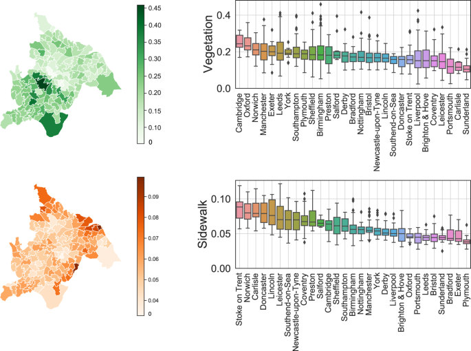
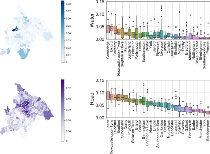
We adopt the deep learning model to mine the semantic information in both street view and satellite view imagery. To ensure the reliability of the generated features, several quality control procedures are adopted. First, we choose the state-of-the-art deep learning model that ranks first for unseen images in the segmentation task. The standardized benchmarks in the computer vision community ensure the reliability of model selection. Specifically, we use the ViT-Adapter model55 for both street view and satellite view images, which leverages the recent advances in vision transformer77 to greatly improve the accuracy and generalizability of semantic segmentation models. Second, we select the training dataset that includes varying scenarios to enhance the transferability of the model. For street view image segmentation, we use the Cityscapes dataset57, which is one of the standard datasets for segmentation tasks. It contains 25000 annotated urban street scenes for 50 different cities in a variety of seasons, daytime, and weather conditions. For satellite view segmentation, we choose the famous LoveDA dataset61 that contains 5987 high spatial resolution satellite images for 18 different administrative districts in both urban and rural areas. The wide coverage of training data helps the model to provide reliable results and ensures a successful transfer to images of the UK, which is shown in Fig. 4. Third, for hyperparameters of the model, we use the official implementation provided by the author of ViT-Adapter, where extensive parameter searching and training tricks have been done to make the model rank first. Specifically, AdamW optimizer with an initial learning rate of 2e−5 and weight decay of 0.05 is used to train the model. The full hyperparameter table can be found through the GitHub repository78. Through these parameter combinations, the inference performance achieves a high all pixel accuracy (aAcc) of 97.02% and mean intersection over union (mIoU) of 84.46% for unseen street view images. For the satellite view images, we achieve high performance with aAcc of 71.11% and mIoU of 52.73%, surpassing the state-of-the-art model with mIoU of 52.44%79. Fourth, we further examine the extracted features by human experts to preclude possible defects. For street view segmentation, we visualize the calculated features of vegetation and sidewalk from both the MSOA level and city level and provide an example in Fig. 5. For the satellite view segmentation, we showcase the extracted water and road percentage in Fig. 6.
Visualization of extracted features from street view images. We demonstrate the MSOA level vegetation and sidewalk indicators in Birmingham, and city level distribution in all city-of-interests. The box demonstrates the median and quartiles of the data, and the whiskers extend represent the rest of the distribution (except the outliers).
Visualization of extracted features from satellite view images. We demonstrate the MSOA level water and road indicators in Birmingham, and city level distribution in all city-of-interests. The box demonstrates the median and quartiles of the data, and the whiskers extend represent the rest of the distribution (except the outliers).
Experiments to examine environmental factors with health outcomes
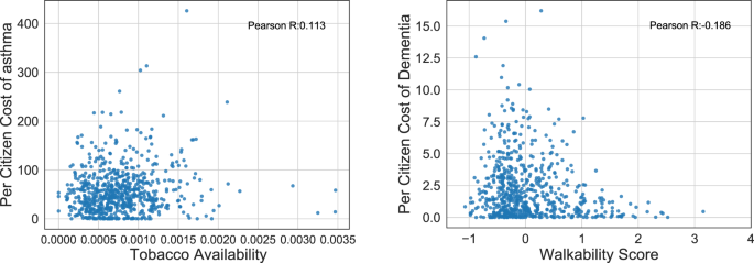
We design some experiments to verify the proposed environmental factors with health outcomes in our dataset, according to the intuition from public health literature. Specifically, the smoking behaviour is positively correlated with asthma incidence80,81,82, while the walking behaviour is negatively correlated with dementia76,83,84. Through our dataset, we use the availability of tobacco POI as the agent for regional level tobacco usage, and the walkability score for walking behaviour. We demonstrate the relationship between the above environmental features with per citizen asthma and dementia expenditure in Fig. 7. We observe a positive correlation of 0.113 for tobacco availability and the cost of asthma, and a negative correlation of −0.186 for walkability and dementia. These observations are consistent with the existing studies, validating the effectiveness of the produced dataset.
Usage Notes
There are several limitations in the present work. First, the definition of “environment” can be broad: from the concrete concept of neighbourhoods for daily living53, to the abstract social and cultural atmosphere85, all these environments could affect public health. Considering the wide range of associations between health and other factors, we focus on physical environments and their health outcomes as quantifiable indicators, while the impact of other factors might also affect the health outcomes summarized in our work. Second, limited by the varying sample frequency of the raw data, we cannot merge the data into a unified time resolution. For instance, the temperature data is daily updated, while the house price is summarized quarterly. Therefore, researchers should be aware that the temporal differences between data records might affect their findings. Third, we use pre-trained semantic segmentation models on standard benchmarks (e.g., Cityscapes) to extract the imagery features from street view and satellite images in the UK, where the accuracy might fluctuate due to the generalizability of the deep learning method. By carefully choosing training benchmarks with high diversity and validating the extracted features, the semantic segmentation models provide reasonable results on UK images and ensure the reliability of the dataset. Researchers should be aware of the scope and limitations of our dataset to make informed judgements on the relationship between environmental determinants and public health.
Code availability
The Python codes to generate the dataset are publicly available through the GitHub repository (https://github.com/0oshowero0/HealthyCities). Detailed instruction for software environment preparation, folder structure and commands to run the provided codes is available in the repository.
References
-
World Health Organization. Integrating health in urban and territorial planning: a sourcebook. https://unhabitat.org/sites/default/files/2020/05/1-final_highres_20002_integrating_health_in_urban_and_territorial_planning_a_sourcebook.pdf (2020).
-
World Health Organization. Compendium of WHO and other UN guidance on health and environment, 2022 update. https://www.who.int/publications/i/item/WHO-HEP-ECH-EHD-22.01 (2022).
-
Galea, S. & Vlahov, D. Urban health: evidence, challenges, and directions. Annu. Rev Public Health 26, 341–365 (2005).
-
Salgado, M. et al. Environmental determinants of population health in urban settings. a systematic review. BMC Public Health 20, 1–11 (2020).
-
Wang, H., Tang, R. & Liu, Y. Potential health benefit of NO2 abatement in China’s urban areas: Inspirations for source-specific pollution control strategy. Lancet Reg Health West Pac 24, 1–2 (2022).
-
Van Daalen, K. et al. The 2022 Europe report of the Lancet Countdown on health and climate change: towards a climate resilient future. Lancet Public Health 7, E942–E965 (2022).
-
Abi Deivanayagam, T. et al. Climate change, health, and discrimination: action towards racial justice. Lancet 401, 5–7 (2023).
-
Watts, N. et al. Health and climate change: policy responses to protect public health. Lancet 386, 1861–1914 (2015).
-
Lee, A. C. K. & Maheswaran, R. The health benefits of urban green spaces: a review of the evidence. Journal of Public Health 33, 212–222 (2011).
-
Lennon, M. Green space and the compact city: Planning issues for a ‘new normal’. Cities & Health 5, S212–S215 (2021).
-
Roscoe, C. et al. Associations of private residential gardens versus other greenspace types with cardiovascular and respiratory disease mortality: observational evidence from UK Biobank. Environ Int 167, 107427 (2022).
-
World Health Organization. Urban green spaces: a brief for action. https://apps.who.int/iris/handle/10665/344116 (2017).
-
World Health Organization. WHO global water, sanitation and hygiene: annual report 2021. https://apps.who.int/iris/bitstream/handle/10665/363169/9789240057258-eng.pdf?sequence=1&isAllowed=y (2022).
-
Committee on the Medical Effects of Air Pollutants. The mortality effects of long-term exposure to particulate air pollution in the united kingdom: A report. https://assets.publishing.service.gov.uk/government/uploads/system/uploads/attachment_data/file/304641/COMEAP_mortality_effects_of_long_term_exposure.pdf (2010).
-
Ventriglio, A., Torales, J., Castaldelli-Maia, J. M., De Berardis, D. & Bhugra, D. Urbanization and emerging mental health issues. CNS Spectr 26, 43–50 (2021).
-
Paykel, E., Abbott, R., Jenkins, R., Brugha, T. & Meltzer, H. Urban–rural mental health differences in Great Britain: findings from the National Morbidity Survey. Psychol Med. 30, 269–280 (2000).
-
World Health Organization. Noncommunicable diseases: what municipal authorities, local governments and ministries responsible for urban planning need to know. https://www.who.int/publications/i/item/WHO-NMH-NMA-16.89 (2016).
-
United Nations. Transforming our world: The 2030 agenda for sustainable development. https://sdgs.un.org/publications/transforming-our-world-2030-agenda-sustainable-development-17981 (2015).
-
Ma, S. & Tong, D. Q. Neighborhood emission mapping operation (NEMO): A 1-km anthropogenic emission dataset in the United States. Scientific Data 9, 1–10 (2022).
-
Ulpiani, G. et al. A citizen centred urban network for weather and air quality in australian schools. Scientific Data 9, 1–9 (2022).
-
Reani, M., Lowe, D., Gledson, A., Topping, D. & Jay, C. UK daily meteorology, air quality, and pollen measurements for 2016–2019, with estimates for missing data. Scientific Data 9, 1–12 (2022).
-
James, W. H., Lomax, N. & Birkin, M. Local level estimates of food, drink and tobacco expenditure for Great Britain. Scientific Data 6, 1–14 (2019).
-
Daras, K., Green, M. A., Davies, A., Barr, B. & Singleton, A. Open data on health-related neighbourhood features in Great Britain. Scientific Data 6, 1–10 (2019).
-
UK Biobank. UK Biobank. https://www.ukbiobank.ac.uk/ (2022).
-
Vuong, Q.-H. The (ir) rational consideration of the cost of science in transition economies. Nat Hum Behav 2, 5–5 (2018).
-
Sharifi, A., Khavarian-Garmsir, A. R. & Kummitha, R. K. R. Contributions of smart city solutions and technologies to resilience against the COVID-19 pandemic: a literature review. Sustainability 13, 8018 (2021).
-
Chu, Z., Cheng, M. & Song, M. What determines urban resilience against COVID-19: city size or governance capacity? Sustainable Cities and Society 75, 103304 (2021).
-
United Kindom Government. List of cities. https://www.gov.uk/government/publications/list-of-cities (2022).
-
Office for National Statistics Geography. Major towns and cities (December 2015) boundaries v2. https://geoportal.statistics.gov.uk/datasets/ons::major-towns-and-cities-december-2015-boundaries-v2/about (2015).
-
Boeing, G. et al. Using open data and open-source software to develop spatial indicators of urban design and transport features for achieving healthy and sustainable cities. Lancet Glob Health 10, e907–e918 (2022).
-
Office for National Statistics Geography. Middle layer super output area (2011) to major towns and cities (December 2015) lookup in England and Wales. https://geoportal.statistics.gov.uk/datasets/ons::middle-layer-super-output-area-2011-to-major-towns-and-cities-december-2015-lookup-in-england-and-wales/about (2015).
-
Office for National Statistics Geography. Postcode to output area hierarchy to LTLA to UTLA to region to country (May 2021) lookup in England and Wales. https://geoportal.statistics.gov.uk/datasets/postcode-to-output-area-hierarchy-to-ltla-to-utla-to-region-to-country-may-2021-lookup-in-england-and-wales-1/about (2021).
-
Office for National Statistics. Life expectancy (LE) and healthy life expectancy (HLE) at birth by sex for middle layer super output areas (MSOAs) in England. https://www.ons.gov.uk/peoplepopulationandcommunity/healthandsocialcare/healthandlifeexpectancies/datasets/lifeexpectancyleandhealthylifeexpectancyhleatbirthbysexformiddlelayersuperoutputareasmsoasinengland (2015).
-
NHS Business Service Authority. English prescribing dataset. https://opendata.nhsbsa.net/dataset/english-prescribing-data-epd (2022).
-
NHS Business Service Authority. Open data portal API. https://www.ons.gov.uk/peoplepopulationandcommunity/healthandsocialcare/healthandlifeexpectancies/datasets/lifeexpectancyleandhealthylifeexpectancyhleatbirthbysexformiddlelayersuperoutputareasmsoasinengland (2022).
-
National Institude for Health and Care Excellence. British national formulary (BNF). https://bnf.nice.org.uk/ (2022).
-
UK Government. Coronavirus (COVID-19) in the UK. https://coronavirus.data.gov.uk/ (2022).
-
Office for National Statistics. Middle super output area population estimates. https://www.ons.gov.uk/peoplepopulationandcommunity/populationandmigration/populationestimates/datasets/middlesuperoutputareamidyearpopulationestimates (2020).
-
Office for National Statistics Geography. Middle layer super output areas (December 2011) boundaries generalised clipped (BGC) EW v3. https://geoportal.statistics.gov.uk/datasets/ons::middle-layer-super-output-areas-december-2011-boundaries-generalised-clipped-bgc-ew-v3/about (2011).
-
Office for National Statistics Geography. Middle layer super output areas (December 2011) population weighted centroids. https://geoportal.statistics.gov.uk/datasets/ons::middle-layer-super-output-areas-december-2011-population-weighted-centroids/about (2011).
-
Jimenez, M. P. et al. Residential green space and cognitive function in a large cohort of middle-aged women. JAMA Netw Open. 5, e229306–e229306 (2022).
-
Chavehpour, Y., Rashidian, A., Woldemichael, A. & Takian, A. Inequality in geographical distribution of hospitals and hospital beds in densely populated metropolitan cities of Iran. BMC Health Serv Res. 19, 1–8 (2019).
-
Safegraph. Safegraph places data schema. https://docs.safegraph.com/docs/places (2022).
-
US Census Bureau. North American Industry Classification System (NAICS). https://www.census.gov/naics/ (2017).
-
Adlakha, D. & John, F. The future is urban: integrated planning policies can enable healthy and sustainable cities. Lancet Glob Health 10, e790–e791 (2022).
-
Office for National Statistics. Median house prices by middle layer super output area: HPSSA dataset 2. https://www.ons.gov.uk/peoplepopulationandcommunity/housing/datasets/hpssadataset2medianhousepricebymsoaquarterlyrollingyear (2022).
-
Office for National Statistics. Mean house prices by middle layer super output area: HPSSA dataset 3. https://www.ons.gov.uk/peoplepopulationandcommunity/housing/datasets/hpssadataset3meanhousepricebymsoaquarterlyrollingyear (2022).
-
Office for National Statistics. Median house prices for administrative geographies: HPSSA dataset 9. https://www.ons.gov.uk/peoplepopulationandcommunity/housing/datasets/medianhousepricefornationalandsubnationalgeographiesquarterlyrollingyearhpssadataset09 (2022).
-
Office for National Statistics. Mean house prices for administrative geographies: HPSSA dataset 12. https://www.ons.gov.uk/peoplepopulationandcommunity/housing/datasets/meanhousepricefornationalandsubnationalgeographiesquarterlyrollingyearhpssadataset12 (2022).
-
OpenStreetMap Foundation & Contributors. OpenStreetMap. https://www.openstreetmap.org/ (2022).
-
Geofabrik GmbH, OpenStreetMap Foundation & Contributors. Geofabrik downloads. https://download.geofabrik.de/europe/great-britain/england.html (2022).
-
Google Map. Googe street view. https://www.google.com/maps/ (2022).
-
Nguyen, Q. C. et al. Leveraging 31 million Google street view images to characterize built environments and examine county health outcomes. Public Health Rep 136, 201–211 (2021).
-
Nguyen, Q. C. et al. Using 164 million google street view images to derive built environment predictors of COVID-19 cases. Int J Environ Res Public Health 17, 6359 (2020).
-
Chen, Z. et al. Vision transformer adapter for dense predictions. Preprint at https://arxiv.org/abs/2205.08534 (2022).
-
Chen, Z. et al. The official implementation of the paper “vision transformer adapter for dense predictions”. https://github.com/czczup/vit-adapter (2022).
-
Cordts, M. et al. The cityscapes dataset for semantic urban scene understanding. In Proceedings of the IEEE conference on Computer Vision and Pattern Recognition, 3213–3223 (2016).
-
Esri. World imagery. https://www.arcgis.com/home/item.html?id=10df2279f9684e4a9f6a7f08febac2a9%2F (2022).
-
Han, S. et al. Learning to score economic development from satellite imagery. In Proceedings of the 26th ACM SIGKDD International Conference on Knowledge Discovery & Data Mining, 2970–2979 (2020).
-
Han, S. et al. The official implementation of the paper “learning to score economic development from satellite imagery”. https://github.com/Sungwon-Han/urban_score (2022).
-
Wang, J., Zheng, Z., Ma, A., Lu, X. & Zhong, Y. LoveDA: a remote sensing land-cover dataset for domain adaptive semantic segmentation. In Proceedings of the Neural Information Processing Systems Track on Datasets and Benchmarks, vol. 1 (2021).
-
Frank, L. D. et al. The development of a walkability index: application to the neighborhood quality of life study. British Journal of Sports Medicine 44, 924–933 (2010).
-
Brunekreef, B. & Holgate, S. T. Air pollution and health. Lancet 360, 1233–1242 (2002).
-
Schmitz, O. et al. High resolution annual average air pollution concentration maps for the Netherlands. Scientific Data 6, 1–12 (2019).
-
Reuben, A. et al. Association of air pollution exposure in childhood and adolescence with psychopathology at the transition to adulthood. JAMA Netw Open. 4, e217508–e217508 (2021).
-
UK Air. Automatic urban and rural network. https://uk-air.defra.gov.uk/data/ (2022).
-
UK Air. Interactive monitoring networks map. https://uk-air.defra.gov.uk/interactive-map?network=aurn (2022).
-
UK Air. Site information search. https://uk-air.defra.gov.uk/networks/search-site-info (2022).
-
Suran, M. UN reports new insights on link between climate change and human health. JAMA 327, 2276–2277 (2022).
-
World Health Organization. Climate change and health. https://www.who.int/news-room/fact-sheets/detail/climate-change-and-health (2022).
-
Centers for Disease Control and Prevention. Climate effects on health. https://www.cdc.gov/climateandhealth/effects/default.htm (2022).
-
Burke, M. et al. Higher temperatures increase suicide rates in the United States and Mexico. Nature Climate Change 8, 723–729 (2018).
-
McMichael, A. J. Insights from past millennia into climatic impacts on human health and survival. Proceedings of the National Academy of Sciences 109, 4730–4737 (2012).
-
Met Office. Haduk-grid. https://www.metoffice.gov.uk/research/climate/maps-and-data/data/haduk-grid/haduk-grid (2022).
-
Han, Z., Xia, T., Xi, Y. & Li, Y. Healthy cities: A comprehensive dataset for environmental determinants of health in England cities, figshare, https://doi.org/10.6084/m9.figshare.c.6383148.v1 (2022).
-
Chen, X., Lee, C. & Huang, H. Neighborhood built environment associated with cognition and dementia risk among older adults: a systematic literature review. Soc Sci Med 114560 (2021).
-
Dosovitskiy, A. et al. An image is worth 16 × 16 words: transformers for image recognition at scale. in 2021 International Conference on Learning Representations (ICLR) (2021).
-
Chen, Z. et al. Hyperparameter of “vision transformer adapter for dense predictions”. https://github.com/czczup/ViT-Adapter/blob/main/segmentation/configs/cityscapes/mask2former_beit_adapter_large_896_80k_cityscapes_ss.py (2022).
-
Wang, D. et al. Advancing plain vision transformer towards remote sensing foundation model. IEEE TGRS (2022).
-
Thomson, N., Chaudhuri, R. & Livingston, E. Asthma and cigarette smoking. Eur Respir J 24, 822–833 (2004).
-
McLeish, A. C. & Zvolensky, M. J. Asthma and cigarette smoking: a review of the empirical literature. J Asthma 47, 345–361 (2010).
-
Tiotiu, A., Ioan, I., Wirth, N., Romero-Fernandez, R. & González-Barcala, F.-J. The impact of tobacco smoking on adult asthma outcomes. Int J Environ Res Public Health 18, 992 (2021).
-
Katayama, O. et al. The association between neighborhood amenities and cognitive function: role of lifestyle activities. J Clin Med 9, 2109 (2020).
-
Planalp, E. M. & Okonkwo, O. C. Is 112 the new 10 000?–step count and dementia risk in the uk biobank. JAMA Neurol. 79, 973–974 (2022).
-
Ompad, D. C., Galea, S., Caiaffa, W. T. & Vlahov, D. Social determinants of the health of urban populations: methodologic considerations. J Urban Health. 84, 42–53 (2007).
Acknowledgements
This work was supported in part by the National Key Research and Development Program of China under grant 2020AAA0106000 and the National Natural Science Foundation of China under U1936217. In this work, we use data from the UK government, Office for National Statistics, Department for Environment, Food & Rural Affairs, NHS Business Services Authority, the Met Office, and the Office for Health Improvement and Disparities licensed under the Open Government Licence v.3.0, and the produced dataset contains OS data © Crown copyright and database right [2022]. We use OpenStreetMap data under the Open Data Commons Open Database License 1.0. The satellite image data is collected from Esri under the Esri Master License Agreement. We acknowledge these publicly available data sources for promoting this study.
Author information
Authors and Affiliations
Contributions
Y.L., Z.H. and T.X. contributed in conceptualizing the study. Z.H. acquired raw data, produced the dataset, and prepared all the figures. Y.X. acquired and processed the satellite images. Z.H. contributed to the initial drafting of the manuscript. All authors contributed to data interpretation and critical revision of the manuscript. All authors had full access to all the data in the study and took responsibility for the decision to submit this draft for publication.
Corresponding author
Ethics declarations
Competing interests
The authors declare no competing interests.
Additional information
Publisher’s note Springer Nature remains neutral with regard to jurisdictional claims in published maps and institutional affiliations.
Rights and permissions
Open Access This article is licensed under a Creative Commons Attribution 4.0 International License, which permits use, sharing, adaptation, distribution and reproduction in any medium or format, as long as you give appropriate credit to the original author(s) and the source, provide a link to the Creative Commons license, and indicate if changes were made. The images or other third party material in this article are included in the article’s Creative Commons license, unless indicated otherwise in a credit line to the material. If material is not included in the article’s Creative Commons license and your intended use is not permitted by statutory regulation or exceeds the permitted use, you will need to obtain permission directly from the copyright holder. To view a copy of this license, visit http://creativecommons.org/licenses/by/4.0/.
About this article
Cite this article
Han, Z., Xia, T., Xi, Y. et al. Healthy Cities, A comprehensive dataset for environmental determinants of health in England cities. Sci Data 10, 165 (2023). https://doi.org/10.1038/s41597-023-02060-y
-
Received:
-
Accepted:
-
Published:
-
DOI: https://doi.org/10.1038/s41597-023-02060-y
